Simple example

Here, we show a most basic MBQC proramming using graphix library. In this example, we consider trivial problem of the rotation of two qubits in |0> states. We show how transpiler (Circuit class) can be used, and show the resulting meausrement pattern.

First, let us import relevant modules:

import numpy as np
from graphix import Circuit, Statevec
from graphix.ops import Ops
import networkx as nx
import matplotlib.pyplot as plt

Here, Statevec is our simple statevector simulator class. Next, let us define the problem with a standard quantum circuit. Note that in graphix all qubits starts in |+> states. For this example, we use Hadamard gate (graphix.transpiler.Circuit.h()) to start with |0>

circuit = Circuit(2)

# initialize qubits in |0>, not |+>
circuit.h(1)
circuit.h(0)

# apply rotation gates
theta = np.random.rand(2)
circuit.rx(0, theta[0])
circuit.rx(1, theta[1])

Now we transpile into measurement pattern using transpile() method. This returns Pattern object containing measurement pattern:

pattern = circuit.transpile()
pattern.print_pattern(lim=10)

N, node = 0
N, node = 1
N, node = 2
E, nodes = (1, 2)
M, node = 1, plane = XY, angle(pi) = 0, s-domain = [], t_domain = []
X byproduct, node = 2, domain = [1]
N, node = 3
E, nodes = (0, 3)
M, node = 0, plane = XY, angle(pi) = 0, s-domain = [], t_domain = []
X byproduct, node = 3, domain = [0]
16 more commands truncated. Change lim argument of print_pattern() to show more

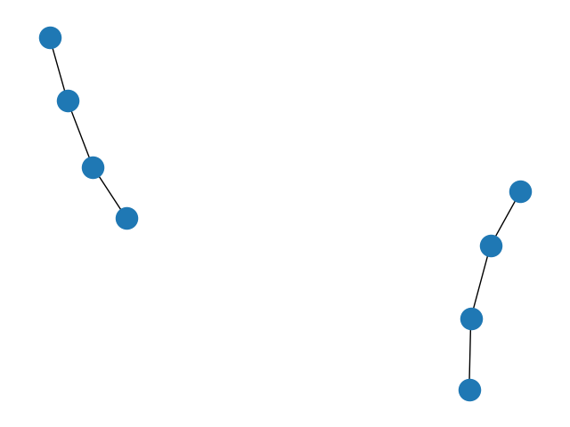
We can plot the graph state to run the above pattern. Since there’s no two-qubit gates applied to the two qubits in the original gate sequence, we see decoupled 1D graphs representing the evolution of single qubits.

nodes, edges = pattern.get_graph()
g = nx.Graph()
g.add_nodes_from(nodes)
g.add_edges_from(edges)
np.random.seed(100)
nx.draw(g)
plt.show()

we can directly simulate the measurement pattern, to obtain the output state.

out_state = pattern.simulate_pattern()
print(out_state.flatten())

[ 0.5694433 -0.60898994j -0.33080966-0.30932751j -0.20271125-0.18954757j
 -0.10296421+0.11011485j]

Let us compare with statevector simulation of the original circuit:

state = Statevec(nqubit=2, plus_states=False)  # starts with |0> states
state.evolve_single(Ops.Rx(theta[0]), 0)
state.evolve_single(Ops.Rx(theta[1]), 1)
print("overlap of states: ", np.abs(np.dot(state.psi.flatten().conjugate(), out_state.psi.flatten())))

overlap of states:  1.0