Minimizing the pattern space

Here, we demonstrate the effect of graphix.pattern.Pattern.minimize_space(). This method reduces the maximum number of qubits that must be prepared at each step of MBQC operation, by delaying the preparation and entanglement of qubits as much as the logical dependency structure allows. This reduces the qubit count (or memory size for classical simulators such as graphix) requirement for any quantum algorithms running on MBQC.

We will demonstrate this by simulating QFT on three qubits. First, import relevant modules and define additional gates we’ll use:

import numpy as np
from graphix import Circuit
import networkx as nx
import matplotlib.pyplot as plt


def cp(circuit, theta, control, target):
    """Controlled phase gate, decomposed"""
    circuit.rz(control, theta / 2)
    circuit.rz(target, theta / 2)
    circuit.cnot(control, target)
    circuit.rz(target, -1 * theta / 2)
    circuit.cnot(control, target)


def swap(circuit, a, b):
    """swap gate, decomposed"""
    circuit.cnot(a, b)
    circuit.cnot(b, a)
    circuit.cnot(a, b)

Now let us define a circuit to apply QFT to three-qubit |011> state (input=6).

circuit = Circuit(3)
for i in range(3):
    circuit.h(i)

# prepare |011> state
circuit.x(1)
circuit.x(2)

# QFT
circuit.h(0)
cp(circuit, np.pi / 2, 1, 0)
cp(circuit, np.pi / 4, 2, 0)
circuit.h(1)
cp(circuit, np.pi / 2, 2, 1)
circuit.h(2)
swap(circuit, 0, 2)

# transpile and plot the graph
pattern = circuit.transpile()
nodes, edges = pattern.get_graph()
g = nx.Graph()
g.add_nodes_from(nodes)
g.add_edges_from(edges)
np.random.seed(100)
nx.draw(g)
plt.show()
print(len(nodes))

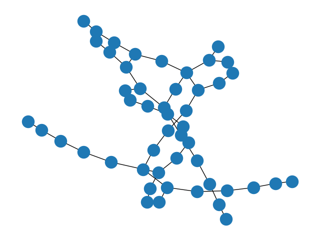
49

This is a graph with 49 qubits, whose statevector is very hard to simulate in ordinary computers. As such, instead of preparing the graph state at the start of the compuation, we opt to prepare qubits as late as possible, so that (destructive) measurements will reduce the burden while we wait. For this, we first standardize and shift signals, to simplify the interdependence of measurements. After that, we can call minimize_space() to perform the optimization.

pattern.standardize()
pattern.shift_signals()
pattern.print_pattern(lim=20)
print(pattern.max_space())

N, node = 0
N, node = 1
N, node = 2
N, node = 3
N, node = 4
N, node = 5
N, node = 6
N, node = 7
N, node = 8
N, node = 9
N, node = 10
N, node = 11
N, node = 12
N, node = 13
N, node = 14
N, node = 15
N, node = 16
N, node = 17
N, node = 18
N, node = 19
136 more commands truncated. Change lim argument of print_pattern() to show more
49

now compare with below:

pattern.minimize_space()
pattern.print_pattern(lim=20)
print(pattern.max_space())

N, node = 0
N, node = 3
E, nodes = (0, 3)
M, node = 0, plane = XY, angle(pi) = 0, s-domain = [], t_domain = []
N, node = 1
N, node = 4
E, nodes = (1, 4)
M, node = 1, plane = XY, angle(pi) = 0, s-domain = [], t_domain = []
N, node = 10
E, nodes = (3, 10)
M, node = 3, plane = XY, angle(pi) = 0, s-domain = [0], t_domain = []
N, node = 6
E, nodes = (4, 6)
M, node = 4, plane = XY, angle(pi) = 0, s-domain = [1], t_domain = []
N, node = 7
E, nodes = (6, 7)
M, node = 6, plane = XY, angle(pi) = -1, s-domain = [], t_domain = []
N, node = 13
E, nodes = (10, 13)
M, node = 10, plane = XY, angle(pi) = -0.25, s-domain = [3], t_domain = []
136 more commands truncated. Change lim argument of print_pattern() to show more
4

The maximum space has gone down to 4 which should be very easily simulated on laptops. Let us check the answer is correct, by comparing with statevector simulation.

out_state = pattern.simulate_pattern()
state = circuit.simulate_statevector()
print("overlap of states: ", np.abs(np.dot(state.psi.flatten().conjugate(), out_state.psi.flatten())))

overlap of states:  0.9999999999999996

Finally, check the output state:

st_expected = [np.exp(2 * np.pi * 1j * 3 * i / 8) / np.sqrt(8) for i in range(8)]
out_stv = out_state.flatten()
print(np.round(st_expected, 3))
print(np.round(out_stv * st_expected[0] / out_stv[0], 3))  # global phase is arbitrary

[ 0.354+0.j    -0.25 +0.25j  -0.   -0.354j  0.25 +0.25j  -0.354+0.j
  0.25 -0.25j   0.   +0.354j -0.25 -0.25j ]
[ 0.354-0.j    -0.25 +0.25j  -0.   -0.354j  0.25 +0.25j  -0.354+0.j
  0.25 -0.25j   0.   +0.354j -0.25 -0.25j ]