Preprocessing Clifford gates

In this example, we implement the Deutsch-Jozsa algorithm which determines whether a function is balanced or constant. Since this algorithm is written only with Clifford gates, we can expect the preprocessing of Clifford gates would significantly improve the MBQC pattern simulation. You can find nice description of the algorithm here.

You can run this code on your browser with mybinder.org - click the badge below.

First, let us import relevant modules:

import numpy as np
from graphix import Circuit
import networkx as nx
import matplotlib.pyplot as plt

Now we implement the algorithm with quantum circuit, which we can transpile into MBQC. As an example, we look at balanced oracle for 4 qubits.

circuit = Circuit(4)

# prepare all qubits in |0> for easier comparison with original algorithm
for i in range(4):
    circuit.h(i)

# initialization
circuit.h(0)
circuit.h(1)
circuit.h(2)

# prepare ancilla
circuit.x(3)
circuit.h(3)

# balanced oracle - flip qubits 0 and 2
circuit.x(0)
circuit.x(2)

# algorithm
circuit.cnot(0, 3)
circuit.cnot(1, 3)
circuit.cnot(2, 3)

circuit.x(0)
circuit.x(2)

circuit.h(0)
circuit.h(1)
circuit.h(2)

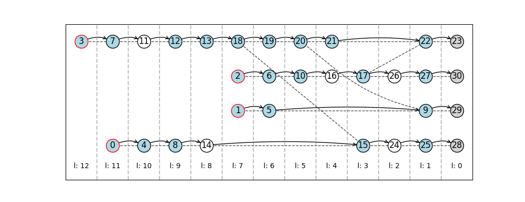
Now let us transpile into MBQC measurement pattern and inspect the pattern sequence and graph state

pattern = circuit.transpile()
pattern.print_pattern(lim=15)
pattern.draw_graph(flow_from_pattern=False)

N, node = 4
E, nodes = (0, 4)
M, node = 0, plane = XY, angle(pi) = 0, s-domain = [], t_domain = []
X byproduct, node = 4, domain = [0]
N, node = 5
E, nodes = (1, 5)
M, node = 1, plane = XY, angle(pi) = 0, s-domain = [], t_domain = []
X byproduct, node = 5, domain = [1]
N, node = 6
E, nodes = (2, 6)
M, node = 2, plane = XY, angle(pi) = 0, s-domain = [], t_domain = []
X byproduct, node = 6, domain = [2]
N, node = 7
E, nodes = (3, 7)
M, node = 3, plane = XY, angle(pi) = 0, s-domain = [], t_domain = []
99 more commands truncated. Change lim argument of print_pattern() to show more
Flow detected in the graph.

this seems to require quite a large graph state. However, we know that Pauli measurements can be preprocessed with graph state simulator. To do so, let us first standardize and shift signals, so that measurements are less interdependent.

pattern.standardize()
pattern.shift_signals()
pattern.print_pattern(lim=15)

N, node = 4
N, node = 5
N, node = 6
N, node = 7
N, node = 8
N, node = 9
N, node = 10
N, node = 11
N, node = 12
N, node = 13
N, node = 14
N, node = 15
N, node = 16
N, node = 17
N, node = 18
77 more commands truncated. Change lim argument of print_pattern() to show more

Now we preprocess all Pauli measurements

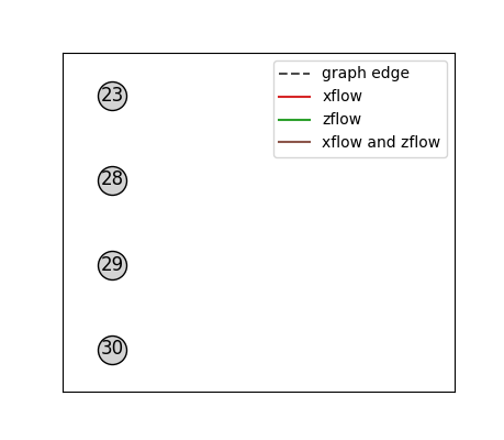
pattern.perform_pauli_measurements()
pattern.print_pattern(lim=16, filter=["N", "M", "C"])
pattern.draw_graph(flow_from_pattern=True)

N, node = 23
N, node = 28
N, node = 29
N, node = 30
Clifford, node = 28, Clifford index = 8
Clifford, node = 29, Clifford index = 8
Clifford, node = 30, Clifford index = 8
Clifford, node = 23, Clifford index = 3
The pattern is not consistent with flow or gflow structure.

Since all operations of the original circuit are Clifford, all measurements in the measurement pattern are Pauli measurements: So the preprocessing has done all the necessary computations, and all nodes are isolated with no further measurements required. Let us make sure the result is correct:

out_state = pattern.simulate_pattern()
state = circuit.simulate_statevector()
print("overlap of states: ", np.abs(np.dot(state.psi.flatten().conjugate(), out_state.psi.flatten())))

overlap of states:  0.4999999999999996