Statevector simulation of MBQC patterns

Here we benchmark our statevector simulator for MBQC.

The methods and modules we use are the followings:

1. graphix.pattern.Pattern.simulate_pattern()

   Pattern simulator with statevector backend.

2. paddle_quantum.mbqc

   Pattern simulation using paddle_quantum.mbqc.

Firstly, let us import relevant modules:

from time import perf_counter
import matplotlib.pyplot as plt
import numpy as np
from graphix import Circuit
from paddle import to_tensor
from paddle_quantum.mbqc.qobject import Circuit as PaddleCircuit
from paddle_quantum.mbqc.transpiler import transpile as PaddleTranspile
from paddle_quantum.mbqc.simulator import MBQC as PaddleMBQC

/home/docs/checkouts/readthedocs.org/user_builds/graphix/envs/v0.2.11/lib/python3.10/site-packages/setuptools/sandbox.py:14: DeprecationWarning: pkg_resources is deprecated as an API. See https://setuptools.pypa.io/en/latest/pkg_resources.html
  import pkg_resources
/home/docs/checkouts/readthedocs.org/user_builds/graphix/envs/v0.2.11/lib/python3.10/site-packages/pkg_resources/__init__.py:2832: DeprecationWarning: Deprecated call to `pkg_resources.declare_namespace('google')`.
Implementing implicit namespace packages (as specified in PEP 420) is preferred to `pkg_resources.declare_namespace`. See https://setuptools.pypa.io/en/latest/references/keywords.html#keyword-namespace-packages
  declare_namespace(pkg)
/home/docs/checkouts/readthedocs.org/user_builds/graphix/envs/v0.2.11/lib/python3.10/site-packages/pkg_resources/__init__.py:2832: DeprecationWarning: Deprecated call to `pkg_resources.declare_namespace('sphinxcontrib')`.
Implementing implicit namespace packages (as specified in PEP 420) is preferred to `pkg_resources.declare_namespace`. See https://setuptools.pypa.io/en/latest/references/keywords.html#keyword-namespace-packages
  declare_namespace(pkg)

Next, define a circuit to be transpiled into measurement pattern:

def simple_random_circuit(nqubit, depth):
    r"""Generate a test circuit for benchmarking.

    This function generates a circuit with nqubit qubits and depth layers,
    having layers of CNOT and Rz gates with random placements.

    Parameters
    ----------
    nqubit : int
        number of qubits
    depth : int
        number of layers

    Returns
    -------
    circuit : graphix.transpiler.Circuit object
        generated circuit
    """
    qubit_index = [i for i in range(nqubit)]
    circuit = Circuit(nqubit)
    for _ in range(depth):
        np.random.shuffle(qubit_index)
        for j in range(len(qubit_index) // 2):
            circuit.cnot(qubit_index[2 * j], qubit_index[2 * j + 1])
        for j in range(len(qubit_index)):
            circuit.rz(qubit_index[j], 2 * np.pi * np.random.random())
    return circuit

We define the test cases: shallow (depth=1) random circuits, only changing the number of qubits.

DEPTH = 1
test_cases = [i for i in range(2, 22)]
graphix_circuits = {}

pattern_time = []
circuit_time = []

We then run simulations. First, we run the pattern simulation using graphix. For reference, we perform simple statevector simulation of the original gate network. Since transpilation into MBQC involves a significant increase in qubit number, the MBQC simulation is inherently slower as we will see.

for width in test_cases:
    circuit = simple_random_circuit(width, DEPTH)
    graphix_circuits[width] = circuit
    pattern = circuit.transpile()
    pattern.standardize()
    pattern.minimize_space()
    nodes, edges = pattern.get_graph()
    nqubit = len(nodes)
    start = perf_counter()
    pattern.simulate_pattern(max_qubit_num=30)
    end = perf_counter()
    print(f"width: {width}, nqubit: {nqubit}, depth: {DEPTH}, time: {end - start}")
    pattern_time.append(end - start)
    start = perf_counter()
    circuit.simulate_statevector()
    end = perf_counter()
    circuit_time.append(end - start)

width: 2, nqubit: 8, depth: 1, time: 0.0032319870006176643
width: 3, nqubit: 11, depth: 1, time: 0.003985477000242099
width: 4, nqubit: 16, depth: 1, time: 0.006239907999770367
width: 5, nqubit: 19, depth: 1, time: 0.007873208000091836
width: 6, nqubit: 24, depth: 1, time: 0.010005137000916875
width: 7, nqubit: 27, depth: 1, time: 0.011293122999632033
width: 8, nqubit: 32, depth: 1, time: 0.013949361999038956
width: 9, nqubit: 35, depth: 1, time: 0.016652000000249245
width: 10, nqubit: 40, depth: 1, time: 0.019409540998822195
width: 11, nqubit: 43, depth: 1, time: 0.023045650999847567
width: 12, nqubit: 48, depth: 1, time: 0.033026533001248026
width: 13, nqubit: 51, depth: 1, time: 0.09272507400055474
width: 14, nqubit: 56, depth: 1, time: 0.16084014300031413
width: 15, nqubit: 59, depth: 1, time: 0.2804077149994555
width: 16, nqubit: 64, depth: 1, time: 0.5357544920007058
width: 17, nqubit: 67, depth: 1, time: 0.9995612689999689
width: 18, nqubit: 72, depth: 1, time: 2.4035001719985303
width: 19, nqubit: 75, depth: 1, time: 6.819396704999235
width: 20, nqubit: 80, depth: 1, time: 17.282462236000356
width: 21, nqubit: 83, depth: 1, time: 34.15492564499982

Here we benchmark paddle_quantum, using the same original gate network and use paddle_quantum.mbqc module to transpile into a measurement pattern.

def translate_graphix_rc_into_paddle_quantum_circuit(graphix_circuit: Circuit) -> PaddleCircuit:
    """Translate graphix circuit into paddle_quantum circuit.

    Parameters
    ----------
        graphix_circuit : Circuit
            graphix circuit

    Returns
    -------
        paddle_quantum_circuit : PaddleCircuit
            paddle_quantum circuit
    """
    paddle_quantum_circuit = PaddleCircuit(graphix_circuit.width)
    for instr in graphix_circuit.instruction:
        if instr[0] == "CNOT":
            paddle_quantum_circuit.cnot(which_qubits=instr[1])
        elif instr[0] == "Rz":
            paddle_quantum_circuit.rz(which_qubit=instr[1], theta=to_tensor(instr[2], dtype="float64"))
    return paddle_quantum_circuit


test_cases_for_paddle_quantum = [i for i in range(2, 22)]
paddle_quantum_time = []

for width in test_cases_for_paddle_quantum:
    graphix_circuit = graphix_circuits[width]
    paddle_quantum_circuit = translate_graphix_rc_into_paddle_quantum_circuit(graphix_circuit)
    pat = PaddleTranspile(paddle_quantum_circuit)
    mbqc = PaddleMBQC()
    mbqc.set_pattern(pat)
    start = perf_counter()
    mbqc.run_pattern()
    end = perf_counter()
    paddle_quantum_time.append(end - start)

    print(f"width: {width}, depth: {DEPTH}, time: {end - start}")

width: 2, depth: 1, time: 0.02562445600051433
width: 3, depth: 1, time: 0.030512752000504406
width: 4, depth: 1, time: 0.032550661999266595
width: 5, depth: 1, time: 0.029442138000376872
width: 6, depth: 1, time: 0.04066379899995809
width: 7, depth: 1, time: 0.0442548529990745
width: 8, depth: 1, time: 0.05270048399870575
width: 9, depth: 1, time: 0.06078991999856953
width: 10, depth: 1, time: 0.0678535600000032
width: 11, depth: 1, time: 0.07815398300044762
width: 12, depth: 1, time: 0.09698460599975078
width: 13, depth: 1, time: 0.12486831199930748
width: 14, depth: 1, time: 0.14861550000023271
width: 15, depth: 1, time: 0.22405296800025098
width: 16, depth: 1, time: 0.5044116339995526
width: 17, depth: 1, time: 0.8643571930006146
width: 18, depth: 1, time: 1.1222803919990838
width: 19, depth: 1, time: 2.5713630390000617
width: 20, depth: 1, time: 5.084561814999688
width: 21, depth: 1, time: 15.961366520999945

Lastly, we compare the simulation times.

fig = plt.figure()
ax = fig.add_subplot(111)

ax.scatter(
    test_cases, circuit_time, label="direct statevector sim of original gate-based circuit (reference)", marker="x"
)
ax.scatter(test_cases, pattern_time, label="graphix pattern simulator")
ax.scatter(test_cases_for_paddle_quantum, paddle_quantum_time, label="paddle_quantum pattern simulator")
ax.set(
    xlabel="Width of the original circuit",
    ylabel="time (s)",
    yscale="log",
    title="Time to simulate random circuits",
)
fig.legend(bbox_to_anchor=(0.85, 0.9))
fig.show()

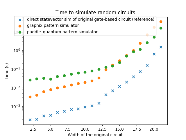
MBQC simulation is a lot slower than the simulation of original gate network, since the number of qubit involved is significantly larger.

import importlib.metadata  # noqa: E402

# print package versions.
[
    print("{} - {}".format(pkg, importlib.metadata.version(pkg)))
    for pkg in ["numpy", "graphix", "paddlepaddle", "paddle-quantum"]
]

numpy - 1.23.5
graphix - 0.2.11
paddlepaddle - 2.4.0rc0
paddle-quantum - 2.2.0

[None, None, None, None]