Graph state simulator backends

Here we benchmark our graph state simulator for MBQC with different backends.

Currently, we have two backends: networkx and rustworkx. Both Python packages are used to manipulate graphs. While networkx is a pure Python package, rustworkx is a Rust package with Python bindings, which is faster than networkx.

Firstly, let us import relevant modules:

from copy import copy
from time import perf_counter

import matplotlib.pyplot as plt
import numpy as np

from graphix import Circuit

Next, define a function to generate random Clifford circuits.

def genpair(n_qubits, count, rng):
    pairs = []
    for i in range(count):
        choice = [j for j in range(n_qubits)]
        x = rng.choice(choice)
        choice.pop(x)
        y = rng.choice(choice)
        pairs.append((x, y))
    return pairs


def random_clifford_circuit(nqubits, depth, seed=42):
    rng = np.random.default_rng(seed)
    circuit = Circuit(nqubits)
    gate_choice = list(range(5))
    for _ in range(depth):
        for j, k in genpair(nqubits, 2, rng):
            circuit.cnot(j, k)
        for j in range(nqubits):
            k = rng.choice(gate_choice)
            if k == 0:  # H
                circuit.h(j)
            elif k == 1:  # S
                circuit.s(j)
            elif k == 2:  # X
                circuit.x(j)
            elif k == 3:  # Z
                circuit.z(j)
            elif k == 4:  # Y
                circuit.y(j)
            else:
                pass
    return circuit

We generate a set of random Clifford circuits with different widths.

DEPTH = 3
test_cases = [i for i in range(2, 300, 10)]
graphix_patterns = {}

for i in test_cases:
    circuit = random_clifford_circuit(i, DEPTH)
    pattern = circuit.transpile()
    pattern.standardize()
    pattern.shift_signals()
    nodes, edges = pattern.get_graph()
    graphix_patterns[i] = (circuit, pattern, len(nodes))

We then run simulations. First, we run the pattern optimization using networkx.

networkx_time = []
networkx_node = []

for width, (circuit, pattern, num_nodes) in graphix_patterns.items():
    pattern_copy = copy(pattern)
    start = perf_counter()
    pattern_copy.perform_pauli_measurements()
    end = perf_counter()
    networkx_node.append(num_nodes)
    print(f"width: {width}, number of nodes: {num_nodes}, depth: {DEPTH}, time: {end - start}")
    networkx_time.append(end - start)

width: 2, number of nodes: 27, depth: 3, time: 0.005199393999646418
width: 12, number of nodes: 107, depth: 3, time: 0.016133236000314355
width: 22, number of nodes: 177, depth: 3, time: 0.027753812000810285
width: 32, number of nodes: 256, depth: 3, time: 0.0399368170001253
width: 42, number of nodes: 319, depth: 3, time: 0.04725111799962178
width: 52, number of nodes: 408, depth: 3, time: 0.062162685999282985
width: 62, number of nodes: 475, depth: 3, time: 0.07172619699849747
width: 72, number of nodes: 550, depth: 3, time: 0.08245711099880282
width: 82, number of nodes: 613, depth: 3, time: 0.09208274699994945
width: 92, number of nodes: 685, depth: 3, time: 0.10312906299986935
width: 102, number of nodes: 760, depth: 3, time: 0.11783187499895575
width: 112, number of nodes: 851, depth: 3, time: 0.13120519100084493
width: 122, number of nodes: 926, depth: 3, time: 0.14155090800159087
width: 132, number of nodes: 998, depth: 3, time: 0.1536988809984905
width: 142, number of nodes: 1070, depth: 3, time: 0.16652637500010314
width: 152, number of nodes: 1148, depth: 3, time: 0.17783746600071026
width: 162, number of nodes: 1222, depth: 3, time: 0.1952539150006487
width: 172, number of nodes: 1303, depth: 3, time: 0.20644108200031042
width: 182, number of nodes: 1383, depth: 3, time: 0.217582264000157
width: 192, number of nodes: 1455, depth: 3, time: 0.2313194319995091
width: 202, number of nodes: 1547, depth: 3, time: 0.24663724300080503
width: 212, number of nodes: 1619, depth: 3, time: 0.2579735660001461
width: 222, number of nodes: 1695, depth: 3, time: 0.2695937709995633
width: 232, number of nodes: 1770, depth: 3, time: 0.28682402100093896
width: 242, number of nodes: 1845, depth: 3, time: 0.30006107600092946
width: 252, number of nodes: 1918, depth: 3, time: 0.3098282780010777
width: 262, number of nodes: 1999, depth: 3, time: 0.3231914030002372
width: 272, number of nodes: 2069, depth: 3, time: 0.33589928099900135
width: 282, number of nodes: 2154, depth: 3, time: 0.35330047699972056
width: 292, number of nodes: 2224, depth: 3, time: 0.3646376649994636

Next, we run the pattern optimization using rustworkx.

rustworkx_time = []
rustworkx_node = []

for width, (circuit, pattern, num_nodes) in graphix_patterns.items():
    pattern_copy = copy(pattern)
    start = perf_counter()
    pattern_copy.perform_pauli_measurements(use_rustworkx=True)
    end = perf_counter()
    rustworkx_node.append(num_nodes)
    print(f"width: {width}, number of nodes: {num_nodes}, depth: {DEPTH}, time: {end - start}")
    rustworkx_time.append(end - start)

width: 2, number of nodes: 27, depth: 3, time: 0.0034268819999851985
width: 12, number of nodes: 107, depth: 3, time: 0.011875451000378234
width: 22, number of nodes: 177, depth: 3, time: 0.019776124001509743
width: 32, number of nodes: 256, depth: 3, time: 0.02859647299919743
width: 42, number of nodes: 319, depth: 3, time: 0.03490925900041475
width: 52, number of nodes: 408, depth: 3, time: 0.046390797000640305
width: 62, number of nodes: 475, depth: 3, time: 0.054012526999940746
width: 72, number of nodes: 550, depth: 3, time: 0.06406224199963617
width: 82, number of nodes: 613, depth: 3, time: 0.07224890199904621
width: 92, number of nodes: 685, depth: 3, time: 0.07953749199987215
width: 102, number of nodes: 760, depth: 3, time: 0.08929010100109736
width: 112, number of nodes: 851, depth: 3, time: 0.10140013199998066
width: 122, number of nodes: 926, depth: 3, time: 0.10986480599967763
width: 132, number of nodes: 998, depth: 3, time: 0.1212796680010797
width: 142, number of nodes: 1070, depth: 3, time: 0.12940900899957342
width: 152, number of nodes: 1148, depth: 3, time: 0.1392382459998771
width: 162, number of nodes: 1222, depth: 3, time: 0.1510060140008136
width: 172, number of nodes: 1303, depth: 3, time: 0.16360881499895186
width: 182, number of nodes: 1383, depth: 3, time: 0.17452004199913063
width: 192, number of nodes: 1455, depth: 3, time: 0.18672972900094464
width: 202, number of nodes: 1547, depth: 3, time: 0.20049299099991913
width: 212, number of nodes: 1619, depth: 3, time: 0.20870730499882484
width: 222, number of nodes: 1695, depth: 3, time: 0.22633097600009933
width: 232, number of nodes: 1770, depth: 3, time: 0.233358978999604
width: 242, number of nodes: 1845, depth: 3, time: 0.24428349600020738
width: 252, number of nodes: 1918, depth: 3, time: 0.26074697600051877
width: 262, number of nodes: 1999, depth: 3, time: 0.27052262899997004
width: 272, number of nodes: 2069, depth: 3, time: 0.2806860450000386
width: 282, number of nodes: 2154, depth: 3, time: 0.29708832600044843
width: 292, number of nodes: 2224, depth: 3, time: 0.31049026799882995

Lastly, we compare the simulation times.

assert networkx_node == rustworkx_node

fig = plt.figure()
ax = fig.add_subplot(111)

ax.scatter(networkx_node, networkx_time, label="networkx", color="blue")
ax.scatter(rustworkx_node, rustworkx_time, label="rustworkx", color="red")
ax.set(
    xlabel="Number of nodes in the graph state",
    xscale="log",
    ylabel="Time (s)",
    yscale="log",
    title="Time to perform Pauli measurements on the graph state",
)
ax.legend()
fig.show()

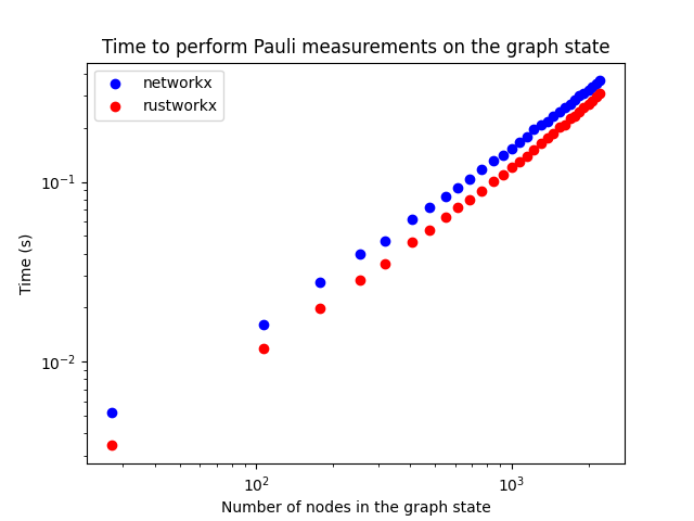
Performing pattern optimization using rustworkx is slightly faster than networkx.

import importlib.metadata  # noqa: E402

# print package versions.
for pkg in ["graphix", "networkx", "rustworkx"]:
    print("{} - {}".format(pkg, importlib.metadata.version(pkg)))

graphix - 0.2.11
networkx - 3.2.1
rustworkx - 0.13.2