Simple example & visualizing graphs

Here, we show a most basic MBQC proramming using graphix library. In this example, we consider trivial problem of the rotation of two qubits in |0> states. We show how transpiler (Circuit class) can be used, and show the resulting meausrement pattern.

In the next example, we describe our visualization tool GraphVisualizer and how to understand the plot.

First, let us import relevant modules:

import numpy as np
from graphix import Circuit, Statevec
from graphix.ops import Ops
import matplotlib.pyplot as plt

Here, Statevec is our simple statevector simulator class. Next, let us define the problem with a standard quantum circuit. Note that in graphix all qubits starts in |+> states. For this example, we use Hadamard gate (graphix.transpiler.Circuit.h()) to start with |0> states instead.

circuit = Circuit(2)

# initialize qubits in |0>, not |+>
circuit.h(1)
circuit.h(0)

# apply rotation gates
theta = np.random.rand(2)
circuit.rx(0, theta[0])
circuit.rx(1, theta[1])

Now we transpile into measurement pattern using transpile() method. This returns Pattern object containing measurement pattern:

pattern = circuit.transpile()
pattern.print_pattern(lim=10)

N, node = 0
N, node = 1
N, node = 2
E, nodes = (1, 2)
M, node = 1, plane = XY, angle(pi) = 0, s-domain = [], t_domain = []
X byproduct, node = 2, domain = [1]
N, node = 3
E, nodes = (0, 3)
M, node = 0, plane = XY, angle(pi) = 0, s-domain = [], t_domain = []
X byproduct, node = 3, domain = [0]
16 more commands truncated. Change lim argument of print_pattern() to show more

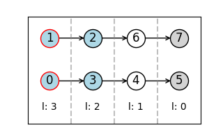
We can plot the graph state to run the above pattern. Since there’s no two-qubit gates applied to the two qubits in the original gate sequence, we see decoupled 1D graphs representing the evolution of single qubits. The arrows are the information flow of the MBQC pattern, obtained using the flow-finding algorithm implemented in graphix.gflow.flow. Below we list the meaning of the node boundary and face colors.

• Nodes with red boundaries are the input nodes where the computation starts.

• Nodes with gray color is the output nodes where the final state end up in.

• Nodes with blue color is the nodes that are measured in Pauli basis, one of X, Y or Z computational bases.

• Nodes in white are the ones measured in non-Pauli basis.

pattern.draw_graph()

Flow found.

we can directly simulate the measurement pattern, to obtain the output state. Internally, we are executing the command sequence we inspected above on a statevector simulator. We also have a tensornetwork simulation backend to handle larger MBQC patterns. see other examples for how to use it.

out_state = pattern.simulate_pattern(backend='statevector')
print(out_state.flatten())

[ 0.99251302-0.06576108j -0.00646952-0.09764254j -0.00209869-0.03167499j
 -0.00311616+0.00020647j]

Let us compare with statevector simulation of the original circuit:

state = Statevec(nqubit=2, plus_states=False)  # starts with |0> states
state.evolve_single(Ops.Rx(theta[0]), 0)
state.evolve_single(Ops.Rx(theta[1]), 1)
print("overlap of states: ", np.abs(np.dot(state.psi.flatten().conjugate(), out_state.psi.flatten())))

overlap of states:  1.0000000000000002

Now let us compile more complex pattern and inspect the graph using the visualization tool. Here, the additional edges with dotted lines are the ones that correspond to CNOT gates, which creates entanglement between the 1D clusters (nodes connected with directed edges) corresponding to the time evolution of a single qubit in the original circuit.

circuit = Circuit(2)

# apply rotation gates
theta = np.random.rand(4)
circuit.rz(0, theta[0])
circuit.rz(1, theta[1])
circuit.cnot(0, 1)
circuit.s(0)
circuit.cnot(1, 0)
circuit.rz(1, theta[2])
circuit.cnot(1, 0)
circuit.rz(0, theta[3])

pattern = circuit.transpile()
pattern.draw_graph()

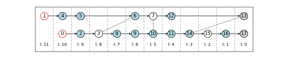
Flow found.