Note
Click here to download the full example code
Quantum classifier with MBQC
In this example, we run data re-uploading quantum cir1cuit from Quantum 4, 226 (2020) to perform binary classification of circles dataset from sklearn.
Firstly, let us import relevant modules:
from graphix.transpiler import Circuit
import networkx as nx
import numpy as np
import matplotlib.pyplot as plt
from sklearn.datasets import make_circles
from scipy.optimize import minimize
from functools import reduce
import seaborn as sns
from matplotlib import cm
from IPython.display import clear_output
from time import time

np.random.seed(0)
Dataset
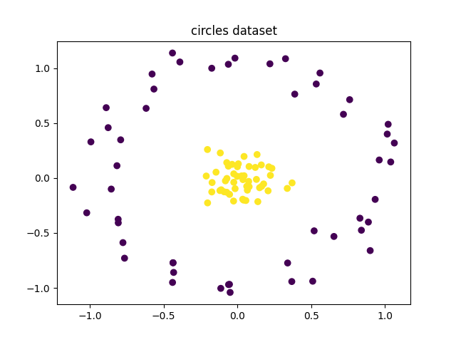
Generate circles dataset with arge circle containing a smaller circle in 2d. The dataset is padded with zeros to make it compatible with the quantum circuit. We want the number of features to be a multiple of 3 as the quantum circuit uses 3 features at a time with gates \(R_x, R_y, R_z\). We also change the labels to -1 and 1 as later we will use Pauli Z operator for measurment whose expectation values are \(\pm 1\).
x, y = make_circles(n_samples=100, noise=0.1, factor=0.1, random_state=32)

# Plot the circle pattern
plt.scatter(x[:, 0], x[:, 1], c=y)
plt.title('circles dataset')
plt.show()

# pad data
x = np.pad(x, ((0, 0), (0, 1)))

# hinge labels
y = 2*y - 1
x.shape, y.shape
((100, 3), (100,))
QNN Class with Graphix
We define a class for the quantum neural network which uses the data re-uploading quantum circuit.
class QNN:
def __init__(self, n_qubits, n_layers, n_features):
"""
Initialize uantum neural network with a specified number of
qubits, layers, and features.
Args:
n_qubits: The number of qubits in the quantum circuit.
n_layers: The number of layers in the quantum circuit.
n_features: The number of features used in the quantum circuit.
It must be a multiple of 3.
"""
super().__init__()
self.n_qubits = n_qubits
self.n_layers = n_layers
self.n_features = n_features
assert n_features % 3 == 0, "n_features must be a multiple of 3"
# Pauli Z operator on all qubits
Z_OP = np.array([[1, 0],
[0, -1]])
operator = [Z_OP]*self.n_qubits
self.obs = reduce(np.kron, operator)
self.cost_values = [] # to store cost values during optimization
def rotation_layer(self, circuit, qubit, params, input_params):
"""
Apply otation gates around the x, y, and z axes to a specified qubit in a
quantum circuit.
Args:
circuit: The quantum circuit on which the rotation layer is applied.
qubit: The qubit on which the rotation gates are applied.
params: The `params` variable is a 2D numpy array with shape `(3, 2)`.
input_params: Feature vector of shape `(3,)`.
"""
z = params[:, 0]*input_params + params[:, 1]
circuit.rx(qubit, z[0])
circuit.ry(qubit, z[1])
circuit.rz(qubit, z[2])
def entangling_layer(self, circuit, n_qubits):
"""
Linear entanglement between qubits in a given circuit.
Args:
circuit: The quantum circuit object that the entangling layer will be added to.
n_qubits: The number of qubits in the quantum circuit.
Returns:
If `n_qubits` is less than 2, nothing is returned. Otherwise, the function
performs a linear entanglement operation on the `n_qubits` qubits in the
given `circuit` using CNOT gates and does not return anything.
"""
if n_qubits < 2:
return
# Linear entanglement
for i in range(n_qubits - 1):
circuit.cnot(i, i + 1)
def data_reuploading_circuit(self, input_params, params):
"""
Creates a data re-uploading quantum circuit using the given input parameters and
parameters for rotation and entangling layers.
Args:
input_params: The input data to be encoded in the quantum circuit. It is a 1D
numpy array of shape `(n_features,)`, where n_features is the number of features
in the input data.
params: The `params` parameter is a flattened numpy array containing the values
of the trainable parameters of the quantum circuit. These parameters are used to
construct the circuit by reshaping them into a 4-dimensional array of shape
`(n_layers, n_qubits, n_features, 2)` where `n_layers` is the number of layers in
the quantum circuit, `n_qubits` is the number of qubits in the quantum circuit,
`n_features` is the number of features in the input data.
Returns:
a quantum circuit object that has been constructed using the input parameters
and the parameters passed to the function.
"""
thetas = params.reshape(self.n_layers, self.n_qubits, self.n_features, 2)
circuit = Circuit(self.n_qubits)
for l in range(self.n_layers):
for f in range(self.n_features//3):
for q in range(self.n_qubits):
self.rotation_layer(circuit,
q,
thetas[l][q][3*f:3*(f+1)],
input_params[3*f:3*(f+1)])
# Entangling layer
if l < self.n_layers -1:
self.entangling_layer(circuit, self.n_qubits)
return circuit
def get_expectation_value(self, sv):
"""
Calculates the expectation value of an PauliZ obeservable given a state vector.
Args:
sv: sSate vector represented as a numpy array.
Returns:
the expectation value of a quantum observable.
"""
exp_val = self.obs@sv
exp_val = np.dot(sv.conj(), exp_val)
return exp_val.real
def compute_expectation(self, data_point, params):
"""
Computes the expectation value of a quantum circuit given a data point and
parameters.
Args:
data_point: Input to the quantum circuit represented as a 1D numpy array.
params: The `params` parameter is a set of parameters that are used to
construct a quantum circuit. The specific details of what these parameters
represent is described in `data_reuploading_circuit` method.
Returns:
the expectation value of a quantum circuit, which is computed using the
statevector of the output state of the circuit.
"""
circuit = self.data_reuploading_circuit(data_point, params)
pattern = circuit.transpile()
pattern.standardize()
pattern.shift_signals()
out_state = pattern.simulate_pattern('tensornetwork')
sv = out_state.to_statevector().flatten()
return self.get_expectation_value(sv)
def cost(self, params, x, y):
"""
Cost function to minimize. The function computes expectation value for each
data point followed by calculating the mean absolute difference between the
predicted and actual values. The cost value is also being appended to a list
called "cost_values"
Args:
params: The `params` parameter is a set of parameters that are used to
construct a quantum circuit. The specific details of what these parameters
represent is described in `data_reuploading_circuit` method.
x: x is a list of input data points used to make predictions.
Each data point is a list or array of features that the model uses to make
a prediction.
y: `y` is a numpy array containing the actual target values for the given
input data `x`. Each value in `y` is either -1 or 1.
Returns:
the cost value
"""
y_pred = [self.compute_expectation(data_point, params) for data_point in x]
cost_val = np.mean(np.abs(y - y_pred))
self.cost_values.append(cost_val)
return cost_val
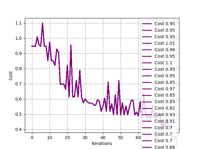
def callback(self, xk):
"""
Plots the cost values against the number of iterations and displays the plot
with the latest cost value as a label.
Args:
xk: `xk` is a parameter that represents the current value of the optimization
variable during the optimization process. It is typically a numpy array or a
list of values. The `callback` function is called at each iteration of the
optimization process and `xk` is passed as an argument to the function.
"""
clear_output(wait=True)
plt.ylabel('Cost')
plt.xlabel('Iterations')
cost_val = np.round(self.cost_values[-1],2)
plt.plot(self.cost_values, color='purple', lw=2, label=f'Cost {cost_val}')
plt.legend()
plt.grid()
plt.show()
def fit(self, x, y, maxiter=5):
"""
This function fits the QNN using the COBYLA optimization method with a maximum
number of iterations and returns the result.
Args:
x: The input data for the model. It is a numpy array of shape
`(n_samples, n_features)`, where `n_samples` is the number of samples and
`n_features` is the number of features in each sample.
y: `y` is a numpy array containing the actual target values for the given
input data `x`. Each value in `y` is either -1 or 1.
maxiter: Maximum number of iterations that the optimization algorithm will
perform during the training process. Defaults to 5
Returns:
The function `fit` returns the result of the optimization process performed
by the `minimize` function from the `scipy.optimize` module.
"""
params = np.random.rand(self.n_layers*self.n_qubits*self.n_features*2)
res = minimize(self.cost,
params,
args=(x, y),
method='COBYLA',
callback=self.callback,
options = {'maxiter': maxiter, 'disp':True})
return res
Train QNN on Circles dataset
n_qubits = 2
n_layers = 2
n_features = 3

qnn = QNN(n_qubits, n_layers, n_features)

start = time()
result = qnn.fit(x, y, maxiter=80)
end = time()

print("Duration:", end-start)
result
Duration: 475.5540060997009

 message: Maximum number of function evaluations has been exceeded.
 success: False
  status: 2
     fun: 0.412676166787027
       x: [ 1.718e+00  7.590e-01 ...  1.630e+00  9.494e-01]
    nfev: 80
   maxcv: 0.0
Compute predictions on the train data and calculate accuracy
predictions = np.array([qnn.compute_expectation(data_point, result.x) for data_point in x])
predictions[predictions > 0.0] = 1.0
predictions[predictions <= 0.0] = -1.0
print(np.mean(y == predictions))
0.91
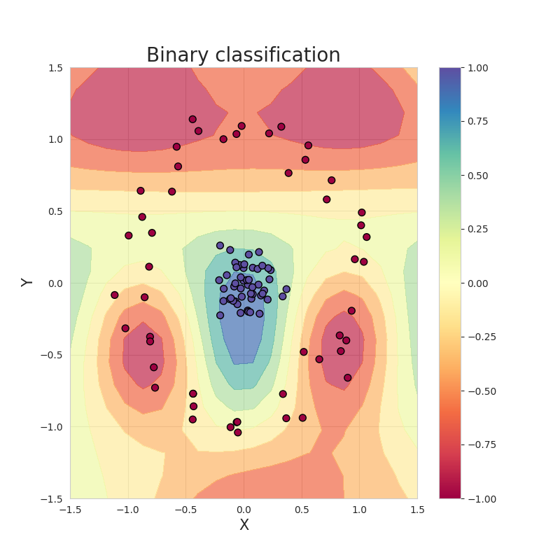
Visualize the decision boundary
We define the grid boundaries and create a meshgrid. We then compute the predictions for each point in the meshgrid and plot the decision boundary.
GRID_X_START = -1.5
GRID_X_END = 1.5
GRID_Y_START = -1.5
GRID_Y_END = 1.5

grid = np.mgrid[GRID_X_START:GRID_X_END:20j,GRID_X_START:GRID_Y_END:20j]
grid_2d = grid.reshape(2, -1).T
XX, YY = grid
grid_2d = np.pad(grid_2d, ((0, 0), (0, 1)))
predictions = np.array([qnn.compute_expectation(data_point, result.x)
                        for data_point in grid_2d])

print(predictions.shape, XX.shape)
(400,) (20, 20)
plt.figure(figsize=(8,8))
sns.set_style("whitegrid")
plt.title('Binary classification', fontsize=20)
plt.xlabel('X', fontsize=15)
plt.ylabel('Y', fontsize=15)
plt.contourf(XX, YY, predictions.reshape(XX.shape), alpha = 0.7, cmap=cm.Spectral)
plt.scatter(x[:, 0], x[:, 1], c=y.ravel(), s=50, cmap=plt.cm.Spectral, edgecolors='black')
plt.colorbar()
plt.show()
Measurement Patterns for the QNN
n_qubits = 2
n_layers = 2
n_features = 3

params = np.random.rand(n_layers * n_qubits * n_features * 2)
input_params = np.random.rand(n_features)

qnn = QNN(n_qubits, n_layers, n_features)
circuit = qnn.data_reuploading_circuit(input_params, params)
pattern = circuit.transpile(opt=False)
pattern.standardize()
pattern.shift_signals()

print(pattern.max_space())
36
Plot the resource state. Node positions are determined by the flow-finding algorithm.
nodes, edges = pattern.get_graph()
g = nx.Graph()
g.add_nodes_from(nodes)
g.add_edges_from(edges)

from graphix.gflow import flow

f, l_k = flow(g, set(range(n_qubits)), set(pattern.output_nodes))

flow = [[i] for i in range(n_qubits)]
for i in range(n_qubits):
    contd = True
    val = i
    while contd:
        try:
            val = f[val]
            flow[i].append(val)
        except KeyError:
            contd = False
longest = np.max([len(flow[i]) for i in range(n_qubits)])

pos = dict()
for i in range(n_qubits):
    length = len(flow[i])
    fac = longest / (length - 1)
    for j in range(len(flow[i])):
        pos[flow[i][j]] = (fac * j, -i)

# determine wheher or not a node will be measured in Pauli basis
def get_clr_list(pattern):
    nodes, edges = pattern.get_graph()
    meas_list = pattern.get_measurement_commands()
    g = nx.Graph()
    g.add_nodes_from(nodes)
    g.add_edges_from(edges)
    clr_list = []
    for i in g.nodes:
        for cmd in meas_list:
            if cmd[1] == i:
                if cmd[3] in [-1, -0.5, 0, 0.5, 1]:
                    clr_list.append([0.5, 0.5, 0.5])
                else:
                    clr_list.append([1, 1, 1])
        if i in pattern.output_nodes:
            clr_list.append([0.8, 0.8, 0.8])
    return clr_list

graph_params = {"with_labels": True,
                "alpha":0.8,
                "node_size": 350,
                "node_color": get_clr_list(pattern),
                "edgecolors": "k"}

nx.draw(g, pos=pos, **graph_params)
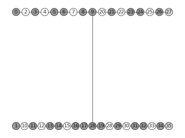
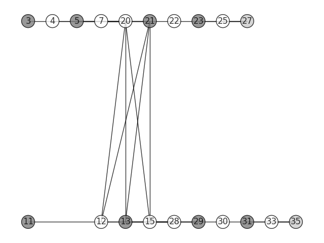
The resource state after Pauli measurement preprocessing:
pattern.perform_pauli_measurements()
nodes, edges = pattern.get_graph()
g = nx.Graph()
g.add_nodes_from(nodes)
g.add_edges_from(edges)
graph_params = {"with_labels": True,
                "alpha":0.8,
                "node_size": 350,
                "node_color": get_clr_list(pattern),
                "edgecolors": "k"}

pos = { # hand-typed for better look
    3: (0,0),
    4: (1,0),
    5: (2,0),
    7: (3,0),
    11: (0,-1),
    12: (3,-1),
    13: (4,-1),
    15: (5,-1),
    20: (4,0),
    21: (5,0),
    22: (6,0),
    23: (7,0),
    25: (8,0),
    27: (9,0),
    28: (6,-1),
    29: (7,-1),
    30: (8,-1),
    31: (9,-1),
    33: (10,-1),
    35: (11,-1),
}

nx.draw(g, pos=pos, **graph_params)
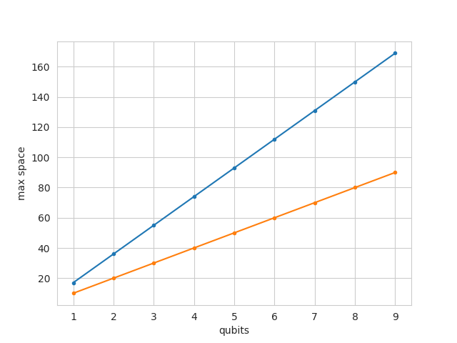
Qubit Resource plot
qubits = range(1, 10)
n_layers = 2
n_features = 3
input_params = np.random.rand(n_features)

before_meas = []
after_meas = []

for n_qubits in qubits:

    params = np.random.rand(n_layers * n_qubits * n_features * 2)
    qnn = QNN(n_qubits, n_layers, n_features)
    circuit = qnn.data_reuploading_circuit(input_params, params)
    pattern = circuit.transpile()
    pattern.standardize()
    pattern.shift_signals()

    before_meas.append(pattern.max_space())

    pattern.perform_pauli_measurements()
    after_meas.append(pattern.max_space())

    del circuit, pattern, qnn, params
Resource state size vs circut width
plt.plot(qubits, before_meas, '.-', label='Before Pauli Meas')
plt.plot(qubits, after_meas, '.-', label='After Pauli Meas')
plt.xlabel("qubits")
plt.ylabel("max space")
plt.show()
Total running time of the script: ( 8 minutes 27.409 seconds)