Tutorial

Graphix provides a high-level interface to generate, optimize and classically simulate the measurement-based quantum computing (MBQC).

In this tutorial, we look at how to program MBQC using graphix library. We will explain the basics here along with the code, and you can go to Introduction to MBQC to learn more about the theoretical background of MBQC and Module reference for module references.

Generating measurement patterns

Graphix is centered around the measurement pattern, which is a sequence of commands such as qubit preparation, entanglement and single-qubit measurement commands. The most basic measurement pattern is that for realizing Hadamard gate, which we will use to see how graphix works.

First, install graphix by

>>> pip install graphix

For any gate network, we can use the Circuit class to generate the measurement pattern to realize the unitary evolution.

from graphix.transpiler import Circuit
# apply H gate to a qubit in + state
circuit = Circuit(1)
circuit.h(0)
pattern = circuit.transpile().pattern

the Pattern object contains the sequence of commands according to the measurement calculus framework [1]. Let us print the pattern (command sequence) that we generated,

>>> pattern.print_pattern() # show the command sequence (pattern)
N, node = 1
E, nodes = (0, 1)
M, node = 0, plane = XY, angle(pi) = 0, s-domain = [], t_domain = []
X byproduct, node = 1, domain = [0]

The command sequence represents the following sequence:

• starting with an input qubit \(|\psi_{in}\rangle_0\), we first prepare an ancilla qubit \(|+\rangle_1\) with [‘N’, 1] command

• We then apply CZ-gate by [‘E’, (0, 1)] command to create entanglement.

• We measure the qubit 0 in Pauli X basis, by [‘M’] command.

• If the measurement outcome is \(s_0 = 1\) (i.e. if the qubit is projected to \(|-\rangle\), the Pauli X eigenstate with eigenvalue of \((-1)^{s_0} = -1\)), the ‘X’ command is applied to qubit 1 to ‘correct’ the measurement byproduct (see Introduction to MBQC) that ensure deterministic computation.

• Tracing out the qubit 0 (since the measurement is destructive), we have \(H|\psi_{in}\rangle_1\) - the input qubit has teleported to qubit 1, while being transformed by Hadamard gate.

This MBQC pattern sequence uses a resource state as shown below:

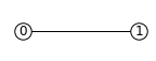
This is the simplest of the graph state with nodes = [0, 1] and edge = (0, 1). Any MBQC pattern has a corresponding resource graph state on which the computation occurs only with single-qubit measurements.

We can use the PatternSimulator to classically simulate the pattern above and obtain the output state, for default input state of \(|+\rangle\). Alternatively, we can simply call simulate_pattern() of Pattern object to do it in one line:

>>> pattern.simulate_pattern(backend='statevector')
Statevec, data=[1.+0.j 0.+0.j], shape=(2,)

Note again that we started with \(|+\rangle\) state so the answer is correct.

We can use the in-built visualization tool to view the pattern,

>>> pattern.draw_graph()

Universal gate sets

As a more complex example than above, we show measurement patterns and graph states for CNOT and single-qubit general rotation which makes MBQC universal:

CNOT

control: input=0, output=0; target: input=1, output=3

>>> cnot_pattern.print_pattern() N, node = 0 N, node = 1 N, node = 2 N, node = 3 E, nodes = (1, 2) E, nodes = (0, 2) E, nodes = (2, 3) M, node = 1, plane = XY, angle(pi) = 0, s-domain = [], t_domain = [] M, node = 2, plane = XY, angle(pi) = 0, s-domain = [], t_domain = [] X byproduct, node = 3, domain = [2] Z byproduct, node = 3, domain = [1] Z byproduct, node = 0, domain = [1]

general rotation (an example with Euler angles 0.2pi, 0.15pi and 0.1 pi)

input = 0, output = 4

>>> euler_rot_pattern.print_pattern() N, node = 0 N, node = 1 N, node = 2 N, node = 3 N, node = 4 M, node = 0, plane = XY, angle(pi) = -0.2, s-domain = [], t_domain = [] M, node = 1, plane = XY, angle(pi) = -0.15, s-domain = [0], t_domain = [] M, node = 2, plane = XY, angle(pi) = -0.1, s-domain = [1], t_domain = [] M, node = 3, plane = XY, angle(pi) = 0, s-domain = [], t_domain = [] Z byproduct, node = 4, domain = [0,2] X byproduct, node = 4, domain = [1,3]

We can concatenate these commands to perform any quantum information processing tasks, which we will look at in more detail below. Of course, we also have many other gates that can be transpiled into MBQC; see Circuit class.

Optimizing patterns

We provide a number of optimization routines to improve the measurement pattern. As an example, let us prepare a pattern to rotate two qubits in \(|+\rangle\) with a random angle and entangle them with a CNOT gate:

from graphix.transpiler import Circuit
import numpy as np
circuit = Circuit(2) # initialize with |+> \otimes |+>
circuit.rz(0, np.random.rand())
circuit.rz(1, np.random.rand())
circuit.cnot(0, 1)
pattern = circuit.transpile().pattern

This produces a rather long and complicated command sequence.

>>> pattern.print_pattern() # show the command sequence (pattern)
N, node = 2
N, node = 3
E, nodes = (0, 2)
E, nodes = (2, 3)
M, node = 0, plane = XY, angle(pi) = -0.2975038024267561, s-domain = [], t_domain = []
M, node = 2, plane = XY, angle(pi) = 0, s-domain = [], t_domain = []
X byproduct, node = 3, domain = [2]
Z byproduct, node = 3, domain = [0]
N, node = 4
N, node = 5
E, nodes = (1, 4)
E, nodes = (4, 5)
M, node = 1, plane = XY, angle(pi) = -0.14788446865973076, s-domain = [], t_domain = []
M, node = 4, plane = XY, angle(pi) = 0, s-domain = [], t_domain = []
X byproduct, node = 5, domain = [4]
Z byproduct, node = 5, domain = [1]
N, node = 6
N, node = 7
E, nodes = (5, 6)
E, nodes = (3, 6)
E, nodes = (6, 7)
M, node = 5, plane = XY, angle(pi) = 0, s-domain = [], t_domain = []
M, node = 6, plane = XY, angle(pi) = 0, s-domain = [], t_domain = []
X byproduct, node = 7, domain = [6]
Z byproduct, node = 7, domain = [5]
Z byproduct, node = 3, domain = [5]

As we see below, we can simplify and optimize the pattern by calling various methods of Pattern.

Standardization and signal shifting

The standard pattern is a pattern where the commands are sorted in the order of N, E, M, (X, Z, C) where X, Z and C commands in bracket can be in any order but must apply only to output nodes. Any command sequence has a standard form, which can be obtained by the standardization algorithm in [1] that runs in polynomial time on the number of commands.

An additional signal shifting procedure simplifies the dependence structure of the pattern to minimize the feedforward operations. These can be called with standardize() and shift_signals() and result in a simpler pattern sequence.

>>> pattern.standardize()
>>> pattern.shift_signals()
>>> pattern.print_pattern()
N, node = 2
N, node = 3
N, node = 4
N, node = 5
N, node = 6
N, node = 7
E, nodes = (0, 2)
E, nodes = (2, 3)
E, nodes = (1, 4)
E, nodes = (4, 5)
E, nodes = (5, 6)
E, nodes = (6, 3)
E, nodes = (6, 7)
M, node = 0, plane = XY, angle(pi) = -0.2975038024267561, s-domain = [], t_domain = []
M, node = 2, plane = XY, angle(pi) = 0, s-domain = [], t_domain = []
M, node = 1, plane = XY, angle(pi) = -0.14788446865973076, s-domain = [], t_domain = []
M, node = 4, plane = XY, angle(pi) = 0, s-domain = [], t_domain = []
M, node = 5, plane = XY, angle(pi) = 0, s-domain = [4], t_domain = []
M, node = 6, plane = XY, angle(pi) = 0, s-domain = [], t_domain = []
X byproduct, node = 3, domain = [2]
X byproduct, node = 7, domain = [2, 4, 6]
Z byproduct, node = 3, domain = [0, 1, 5]
Z byproduct, node = 7, domain = [1, 5]

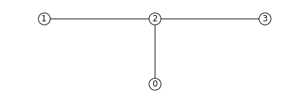
The command sequence is now simpler and note that the most byproduct commands now apply to output nodes (3, 7). This reveals the graph structure of the resource state which we can inspect:

import networkx as nx
nodes, edges = pattern.get_graph()
g = nx.Graph()
g.add_nodes_from(nodes)
g.add_edges_from(edges)
pos = {0: (0, 0), 1: (0, -0.5), 2: (1, 0), 3: (4, 0), 4: (1, -0.5), 5: (2, -0.5), 6: (3, -0.5), 7: (4, -0.5)}
graph_params = {'node_size': 240, 'node_color': 'w', 'edgecolors': 'k', 'with_labels': True}
nx.draw(g, pos=pos, **graph_params)

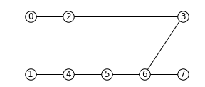
0 and 1 are the input nodes and 3 and 7 are the output nodes of this graph.

Performing Pauli measurements

It is known that quantum circuit consisting of Pauli basis states, Clifford gates and Pauli measurements can be simulated classically (see Gottesman-Knill theorem; e.g. the graph state simulator runs in \(\mathcal{O}(n \log n)\) time). The Pauli measurement part of the MBQC is exactly this, and they can be preprocessed by our graph state simulator GraphState - see Introduction to LC-MBQC for more detailed description.

We can call this in a line by calling perform_pauli_measurements() of Pattern object, which acts as the optimization routine of the measurement pattern. We get an updated measurement pattern without Pauli measurements as follows:

>>> pattern.perform_pauli_measurements()
>>> pattern.print_pattern()
N, node = 3
N, node = 7
E, nodes = (0, 3)
E, nodes = (1, 3)
E, nodes = (1, 7)
M, node = 0, plane = XY, angle(pi) = -0.2975038024267561, s-domain = [], t_domain = [], Clifford index = 6
M, node = 1, plane = XY, angle(pi) = -0.14788446865973076, s-domain = [], t_domain = [], Clifford index = 6
X byproduct, node = 3, domain = [2]
X byproduct, node = 7, domain = [2, 4, 6]
Z byproduct, node = 3, domain = [0, 1, 5]
Z byproduct, node = 7, domain = [1, 5]

Notice that all measurements with angle=0 (Pauli X measurements) disappeared - this means that a part of quantum computation was classically (and efficiently) preprocessed such that we only need much smaller quantum resource. The additional Clifford commands, along with byproduct operations, can be dealt with by simply rotating the final readout measurements from the standard Z basis, so there is no downside in doing this preprocessing.

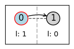
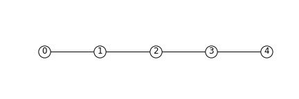
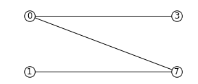
As you can see below, the resource state has shrank significantly (factor of two reduction in the number of nodes), but again we know that they both serve as the quantum resource state for the same quantum computation task as defined above.

before	after

As we mention in Introduction to MBQC, all Clifford gates translates into MBQC only consisting of Pauli measurements. So this procedure is equivalent to classically preprocessing all Clifford operations from quantum algorithms.

Minimizing ‘space’ of a pattern

The space of a pattern is the largest number of qubits that must be present in the graph state during the execution of the pattern. For standard patterns, this is exactly the size of the resource graph state, since we prepare all ancilla qubits at the start of the computation. However, we do not always need to prepare all qubits at the start; in fact preparing all the adjacent (connected) qubits of the ones that you are about measure, is sufficient to run MBQC. We exploit this fact to minimize the space of the pattern, which is crucial for running statevector simulation of MBQC since they are typically limited by the available computer memory. We can simply call minimize_space() to reduce the space:

>>> pattern.minimize_space()
>>> pattern.print_pattern(lim=20)
N, node = 3
E, nodes = (0, 3)
M, node = 0, plane = XY, angle(pi) = -0.2975038024267561, s-domain = [], t_domain = [], Clifford index = 6
E, nodes = (1, 3)
N, node = 7
E, nodes = (1, 7)
M, node = 1, plane = XY, angle(pi) = -0.14788446865973076, s-domain = [], t_domain = [], Clifford index = 6
X byproduct, node = 3, domain = [2]
X byproduct, node = 7, domain = [2, 4, 6]
Z byproduct, node = 3, domain = [0, 1, 5]
Z byproduct, node = 7, domain = [1, 5]

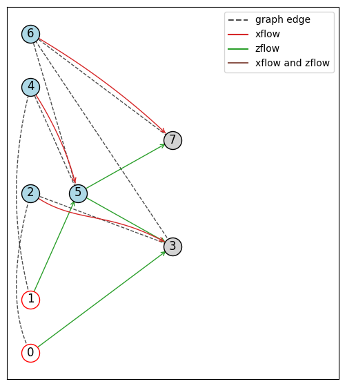
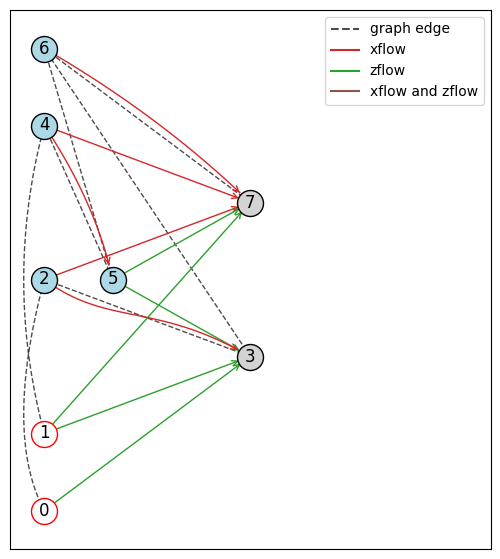
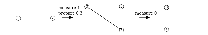
With the original measurement pattern, the simulation should have proceeded as follows, with maximum of four qubits on the memory.

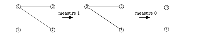
With the optimization with minimize_space(), the simulation proceeds as below, where we measure and trace out qubit 1 before preparing qubits 0 and 3. Because the graph state only has short-range correlations (only adjacent qubits are entangled), this does not affect the outcome of the computation. With this, we only need the memory space for three qubits.

This procedure is more effective when the resource state size is large compared to the logical input qubit count; for example, the three-qubit quantum Fourier transform (QFT) circuit requires 12 qubits in the resource state after perform_pauli_measurements() (see the code in QFT example); with the proper reordering of the commands, the max_space reduces to 4. In fact, for patterns transpiled from gate network, the minimum space we can realize is typically \(n_w+1\) where \(n_w\) is the width of the circuit.

Simulating noisy MBQC

We can simulate the MBQC pattern with various noise models to understand their effects. The pattern that we used above can be simulated with the statevector backend.

out_state = pattern.simulate_pattern(backend="statevector")

With the simulated pattern, we can define a noise model. We specify Kraus channels for each of the command executions, and we apply dephasing noise to the qubit preparation.

from graphix.channels import KrausChannel, dephasing_channel
from graphix.noise_models.noise_model import NoiseModel
from graphix.noise_models.noiseless_noise_model import NoiselessNoiseModel

class NoisyGraphState(NoiseModel):

    def __init__(self, p_z=0.1):
        self.p_z = p_z

    def prepare_qubit(self):
        """return the channel to apply after clean single-qubit preparation. Here just we prepare dephased qubits."""
        return dephasing_channel(self.p_z)

    def entangle(self):
        """return noise model to qubits that happens after the CZ gate. just identity no noise for this noise model."""
        return KrausChannel([{"coef": 1.0, "operator": np.eye(4)}])

    def measure(self):
        """apply noise to qubit to be measured."""
        return KrausChannel([{"coef": 1.0, "operator": np.eye(2)}])

    def confuse_result(self, cmd):
        """imperfect measurement effect. here we do nothing (no error).
        cmd = "M"
        """
        pass

    def byproduct_x(self):
        """apply noise to qubits after X gate correction. here no error (identity)."""
        return KrausChannel([{"coef": 1.0, "operator": np.eye(2)}])

    def byproduct_z(self):
        """apply noise to qubits after Z gate correction. here no error (identity)."""
        return KrausChannel([{"coef": 1.0, "operator": np.eye(2)}])

    def clifford(self):
        """apply noise to qubits that happens in the Clifford gate process. here no error (identity)."""
        return KrausChannel([{"coef": 1.0, "operator": np.eye(2)}])

    def tick_clock(self):
        """notion of time in real devices - this is where we apply effect of T1 and T2.
        we assume commands that lie between 'T' commands run simultaneously on the device.

        here we assume no idle error.
        """
        pass

With the noise model written, we can simulate it.

from graphix.simulator import PatternSimulator

simulator = PatternSimulator(pattern, backend="densitymatrix", noise_model=NoisyGraphState(p_z=0.01))
dm_result = simulator.run()

>>> print(dm_result.fidelity(out_state.psi.flatten()))
0.9718678141724848

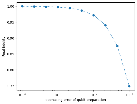
We can plot the results from the model,

import matplotlib.pyplot as plt

err_arr = np.logspace(-4, -1, 10)
fidelity = np.zeros(10)
for i in range(10):
    simulator = PatternSimulator(pattern, backend="densitymatrix", noise_model=NoisyGraphState(p_z=err_arr[i]))
    dm_result = simulator.run()
    fidelity[i] = dm_result.fidelity(out_state.psi.flatten())

plt.semilogx(err_arr, fidelity, "o:")
plt.xlabel("dephasing error of qubit preparation")
plt.ylabel("Final fidelity")
plt.show()

Running pattern on quantum devices

We are currently adding cloud-based quantum devices to run MBQC pattern. Our first such interface is for IBMQ devices, and is available as graphix-ibmq module.

First, install graphix-ibmq by

>>> pip install graphix-ibmq

With graphix-ibmq installed, we can turn a measurement pattern into a qiskit dynamic circuit.

from graphix_ibmq.runner import IBMQBackend

# minimize space and convert to qiskit circuit
pattern.minimize_space()
backend = IBMQBackend(pattern)
backend.to_qiskit()
print(type(backend.circ))

#set the rondom input state
psi = []
for i in range(n):
    psi.append(i.random_statevector(2, seed=100+i))
backend.set_input(psi)

<class 'qiskit.circuit.quantumcircuit.QuantumCircuit'>

This can be run on Aer simulator or IBMQ devices. See documentation page for graphix-ibmq interface for more details, as well as a detailed example showing how to run pattern on IBMQ devices.

Generating QASM file

For other systems, we can generate QASM3 instruction set corresponding to the pattern, following

qasm_inst = pattern.to_qasm3('pattern')

Now check the generated qasm file:

$ cat pattern.qasm

// generated by graphix
OPENQASM 3;
include "stdgates.inc";

// measurement result of qubit q2
bit c2 = 0;

// measurement result of qubit q4
bit c4 = 0;

// measurement result of qubit q5
bit c5 = 0;

// measurement result of qubit q6
bit c6 = 0;

// prepare qubit q3
qubit q3;
h q3;

// entangle qubit q0 and q3
cz q0, q3;

// measure qubit q0
bit c0;
float theta0 = 0;
p(-theta0) q0;
h q0;
c0 = measure q0;
h q0;
p(theta0) q0;

...

References

[1] (1,2)

V. Danos, E Kashefi and P. Panangaden, “The Measurement Calculus”, Journal of the ACM 54, 2 (2007)