Patterns and the measurement calculus
Open graphs and correction strategies give a compact picture of an MBQC computation. To reason about computations more systematically, however, it helps to switch to a more operational language: the measurement calculus [DKP07]. It describes a computation as a sequence of elementary instructions, called commands, of four kinds:
Preparation \(\N_i\): prepare qubit \(i\).
Entanglement \(\E_{ij}\): entangle qubits \(i\) and \(j\).
Measurement \(\M_i^{\lambda,\alpha}\): measure qubit \(i\) destructively in the plane \(\lambda(i) \in \{\XYplane, \XZplane, \YZplane\}\), at angle \(\alpha(i) \in [0, 2\pi)\).
Pauli correction \(\X_i^s\) and \(\Z_i^s\): apply a Pauli correction to qubit \(i\), conditional on a classical bit \(s \in \{0, 1\}\). This bit is the parity \(s = \bigoplus_{j \in D} s_j\) of the outcomes of a set \(D\) of previously measured nodes, called the correction domain.
These commands map directly onto the ingredients we have already met:
\(\N\) and \(\E\) together build the resource graph state.
\(\lambda\) and \(\alpha\) assign a measurement plane and angle to every measured qubit (the set \(O^c\)), exactly as in an open graph.
The Pauli corrections implement the XZ-correction maps defined in the previous tutorial.
The precise meaning of each command is summarised in the table below. The states \(\ket{\pm_{\lambda,\alpha}}\) are the measurement basis states defined in the earlier section on measurements; the two outcomes \(s = 0, 1\) correspond to the signs \(+\) and \(-\).
\(\N_i\) |
\(\E_{ij}\) |
\(\M_i^{\lambda,\alpha}\) |
\(\X_i^s,\ \Z_i^s\) |
|---|---|---|---|
\(\otimes \ketplus\) |
\(CZ_{ij}\) |
\(\bra{\pm_{\lambda(i),\alpha(i)}}\) |
\(X_i^s,\ Z_i^s\) |
As with open graphs, when \(\alpha(i)\) is a Pauli angle, i.e. one of \(\{0, \pi/2, \pi, 3\pi/2\}\), the pair \((\lambda(i), \alpha(i))\) can be replaced by a signed axis \(\pm \Xaxis\), \(\pm \Yaxis\) or \(\pm \Zaxis\).
Patterns
A computation in this formalism is a measurement pattern (or simply pattern). A pattern consists of:
a finite sequence of commands acting on a set of qubits, and
two designated qubit sets, the input and output registers.
Not every sequence of commands makes sense physically, so patterns must satisfy runnability conditions [DKP07]:
A command cannot depend on a measurement outcome that is not yet available.
A command can only act on qubits that have not been measured yet. These qubits must be inputs or must have been already prepared.
Qubits are measured if and only if they are not outputs.
Only non-input qubits are prepared, and they are prepared only once.
Example: the Hadamard gate
The Hadamard gate example from the introduction tutorial has the following pattern representation:
Commands are executed from right to left, so the pattern reads as follows:
\(\N_1\): prepare the output qubit 1 in \(\ket{+}\).
\(\E_{01}\): entangle qubits 0 and 1 with a \(CZ\) gate.
\(\M_0^{X}\): measure the input qubit 0 in the \(\Xaxis\) basis, which yields the outcome \(s_0\).
\(\X_1^{s_0}\): apply an \(X\) correction to qubit 1 if \(s_0 = 1\).
In Graphix, patterns are represented by the Pattern class. The example below directly instantiates the Hadamard pattern by specifying the input qubits and the sequence of commands. The output qubits are inferred from the non-measured qubits.
from graphix import Pattern
from graphix.command import E, M, N, X

pattern = Pattern(input_nodes=[0], cmds=[N(1), E((0, 1)), M(0), X(1, {0})])
print(pattern)
X(1,{0}) M(0) E(0,1) N(1)
Tip
Patterns print as ASCII by default. You can use Pattern.to_unicode() or
Pattern.to_latex() for other formats. All three methods, including
Pattern.to_ascii(), accept the parameter limit to truncate long outputs.
Other printable objects offer the same options.
Once a pattern is built, you can run it with simulate() as we did with the XZ-corrections:
from numpy.random import default_rng
from graphix import BasicStates

rng = default_rng(42)

state = pattern.simulate(input_state=BasicStates.ZERO, rng=rng)
print(state)
sqrt(2)/2(|0> + |1>)
Writing patterns in code
As you saw in the previous examples, measurement calculus commands
have a counterpart in Graphix:
N, E, M,
X and Z. We create one by giving the
indices of the nodes it acts on. For the corrections X and
Z, the correction domain is passed as a set of nodes.
By default, M measures along the \(X\) axis. To choose
another plane and angle, pass any Measurement object.
The example below is a slightly bigger pattern that puts all five commands to work. Note that it has two input qubits, and it also contains an \(\XYplane\)-measurement with angle \(\alpha=3\pi/2\) on node 2:
from graphix import Pattern, Measurement
from graphix.command import E, M, N, X, Z

cmds = [
    N(2), E((0, 2)), M(0),
    N(3), E((2, 3)), X(1, {0}), M(2, Measurement.XY(1.5)),
    E((3, 1)), Z(3, {0}), X(3, {2}), Z(1, {2})]

pattern = Pattern(input_nodes=[0, 1], cmds=cmds)
Patterns can be visualized with the method Pattern.draw(). By default it shows the pattern’s flow, but it is possible to show the XZ-correction maps instead:
from graphix import DrawPatternAnnotations
pattern.draw(annotations=DrawPatternAnnotations.XZCorrections)
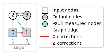
Notice that input qubits can be output qubits too!
The pattern in the example implements a \(R_x(\frac{\pi}{2})\) rotation on qubit 0 followed by a \(CZ\) on qubits 0 and 1. You can try to prove it as an exercise, but don’t worry if it looks too cumbersome. Typically, we don’t instantiate large patterns by hand. In later tutorials, you will learn how to extract patterns from open graphs and how to transpile patterns from circuits.
Pattern standardization
Patterns in the measurement calculus can be manipulated with rewrite rules which allow to absorb a correction into later measurements. This transformation reflects the adaptivity of MBQC: a Pauli correction applied just before a measurement is equivalent to measuring at a modified angle.
Concretely, applying \(\X_i^s \Z_i^t\) to qubit \(i\) right before measuring it gives
where the new angle depends on the measurement plane:
The bits \(s = \bigoplus_{j \in D_s} s_j\) and \(t = \bigoplus_{j \in D_t} s_j\) are called signals. Each one is the parity of earlier measurement outcomes, taken over the sets of measured nodes \(D_s, D_t \subseteq O^c\), which are the domains of the measurement.
In Graphix, an M command stores these domains in its
s_domain and t_domain attributes. As for X and
Z, each domain is given as a set of nodes.
Applying this rule repeatedly, together with the other rules of the calculus [DKP07], allows to bring any pattern into standard form:
all qubit preparations (\(\N\) commands),
then all entanglements (\(\E\) commands),
then all measurements (\(\M\) commands),
and finally the corrections on the output qubits (\(\X\) and \(\Z\) commands).
Graphix implements these rules in Pattern.standardize(). In the example
below, the corrections scattered between the measurements are absorbed into
the measurement domains, leaving only output corrections at the end:
from graphix import Pattern, Measurement
from graphix.command import N, E, M, X, Z

cmds = [
    N(1), N(3), E((0, 3)), N(4), E((0, 4)), E((4, 1)), N(2), E((4, 2)),
    M(0, Measurement.XY(0.3)), X(3, {0}),
    M(2, Measurement.XZ(0.7)), Z(1, {2}), Z(4, {2}), X(3, {2}), X(4, {2}),
    M(1, Measurement.YZ(0.4)), Z(4, {1}),
]

pattern = Pattern(input_nodes=[0], cmds=cmds)
pattern.standardize()
print(pattern)
X(4,{2}) X(3,{0,2}) Z(4,{1,2}) {2}[M(1,YZ,2pi/5)] M(2,XZ,7pi/10) M(0,3pi/10) E(0,3) E(0,4) E(1,4) E(2,4) N(2) N(4) N(3) N(1)
Note
When are two patterns the same?
Pattern’s standard form leaves freedom to arrange commands of the same kind, so it is not a normal form. In Graphix, pattern equality == compares the input, output and commands sequences, so two patterns implementing the same operation may still fail an equality test. In practice, whenever we want to check if two patterns implement the same transformation, we test if they produce the same output state given the same input state up to a global phase. Of course, this only works if the pattern is deterministic, otherwise, you need to compare all possible execution branches.
from graphix import Pattern
from graphix.command import N, E, M, X, Z
from graphix.random_objects import rand_state_vector
from numpy.random import default_rng

rng = default_rng(42)

pattern = Pattern(input_nodes=[0, 1], cmds=[N(2), E((1, 2)), M(1), E((2, 0)), N(3), E((2, 3)), M(2, s_domain={1}), Z(0, {1}), Z(3, {1}), X(3, {2})])

# ``standardize`` acts in place, so we make a copy.
pattern_std = pattern.copy()
pattern_std.standardize()
assert pattern != pattern_std

input_state = rand_state_vector(2, rng=rng)
output_state = pattern.simulate(input_state=input_state, rng=rng)
output_state_std = pattern_std.simulate(input_state=input_state, rng=rng)
assert output_state.isclose(output_state_std)
Clifford commands
Beyond the standard measurement calculus, Graphix adds one command,
\(\C_i\) (C), which applies an unconditional local
Clifford operation to node \(i\). Clifford commands appear as by-products of
certain optimization routines, such as Pauli-measurement removal. They are covered in a dedicated tutorial.
References
Vincent Danos, Elham Kashefi, and Prakash Panangaden. The measurement calculus. J. ACM, 54(2):8–es, apr 2007. URL: https://doi.org/10.1145/1219092.1219096, doi:10.1145/1219092.1219096.